Tunes for the Road
Tuning is one of the most important aspects of programming. It ensures that your mechanisms move smoothly and quickly. It is important to understand how to tune PID control loops by using Pheonix Tuner.
- Plotting and Scheming
- Tuning a CANrange
- Velocity Tuning with VelocityTorqueCurrentFOC
- Shooting Our Shot
- Position Tuning with MotionMagicTorqueCurrentFOC
Plotting and Scheming
Plot (pluh):
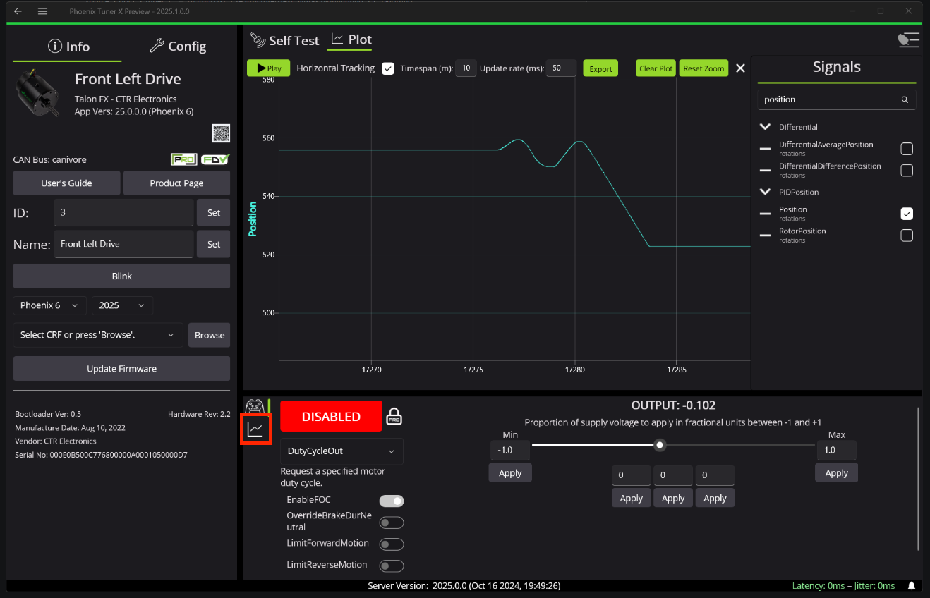
One of the most valuable tools for your tuning endeavors is the Phoenix Tuner plot. The reason this is so useful is that it shows you how much your mechanism is off (in terms of position and velocity) in an intuitive manner.
Read through this guide to understand plotting with Phoenix Tuner:
https://v6.docs.ctr-electronics.com/en/stable/docs/tuner/plotting.html
Signals to Plot (pluh):
-
Position: The actual position of the motor according to the motor (or the CANcoder if there is one)
-
PIDPosition/Reference: The expected position of the motor; The position that you want the motor to be at
-
Velocity: The actual velocity of the motor
-
PIDPosition/Reference Slope: The expected velocity of the motor; The velocity that you want the motor to be at
Plotting Tips:
-
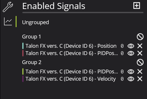
Axis Alignment: One of the most annoying things to deal with when plotting is when the axes for multiple signals are misaligned. To fix this issue, you can group certain signals together. Generally, I put Position and Reference Position in one group and Velocity and Reference Velocity in another.
-
-
In the Phoenix Tuner window, go to the following tab.
-

-
Then, hit the + button to add a new group and drag the signals you want to the correct group.
-
-
-
Presets: It's a good idea to use the three preset boxes to quickly set the target position for the motor at your whim.
Tuning a CANrange
A tuned CANrange is especially important to make sure detection is accurate and reliable!
Read through this guide for some more in depth examples and instructions:
https://v6.docs.ctr-electronics.com/en/latest/docs/application-notes/tuning-canrange.html
CANrange Overview
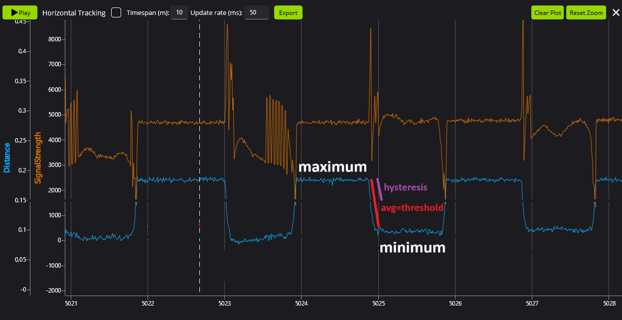
CANranges output many signals to plot in Phoenix Tuner/AScope, however Distance, SignalStrength, and IsDetected are the 3 most important ones:
- Distance is a measure (in meters) of how far an object is from the sensor
- SignalStrength is how accurate the CANrange thinks the distance is
- IsDetected is a true/false boolean (1 for true & 0 for false) of whether the CANrange detects something → dependent on the tuning you will do below
Make sure to add these 3 signals to the plot while tuning!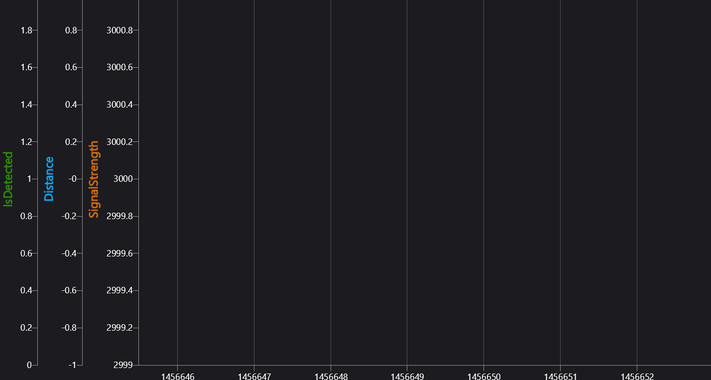
Tuning in Phoenix Tuner
Go to the Config section of the CANrange → the values under the FOV Params & Proximity Params headers are the main values you will be tuning for accurate readings.
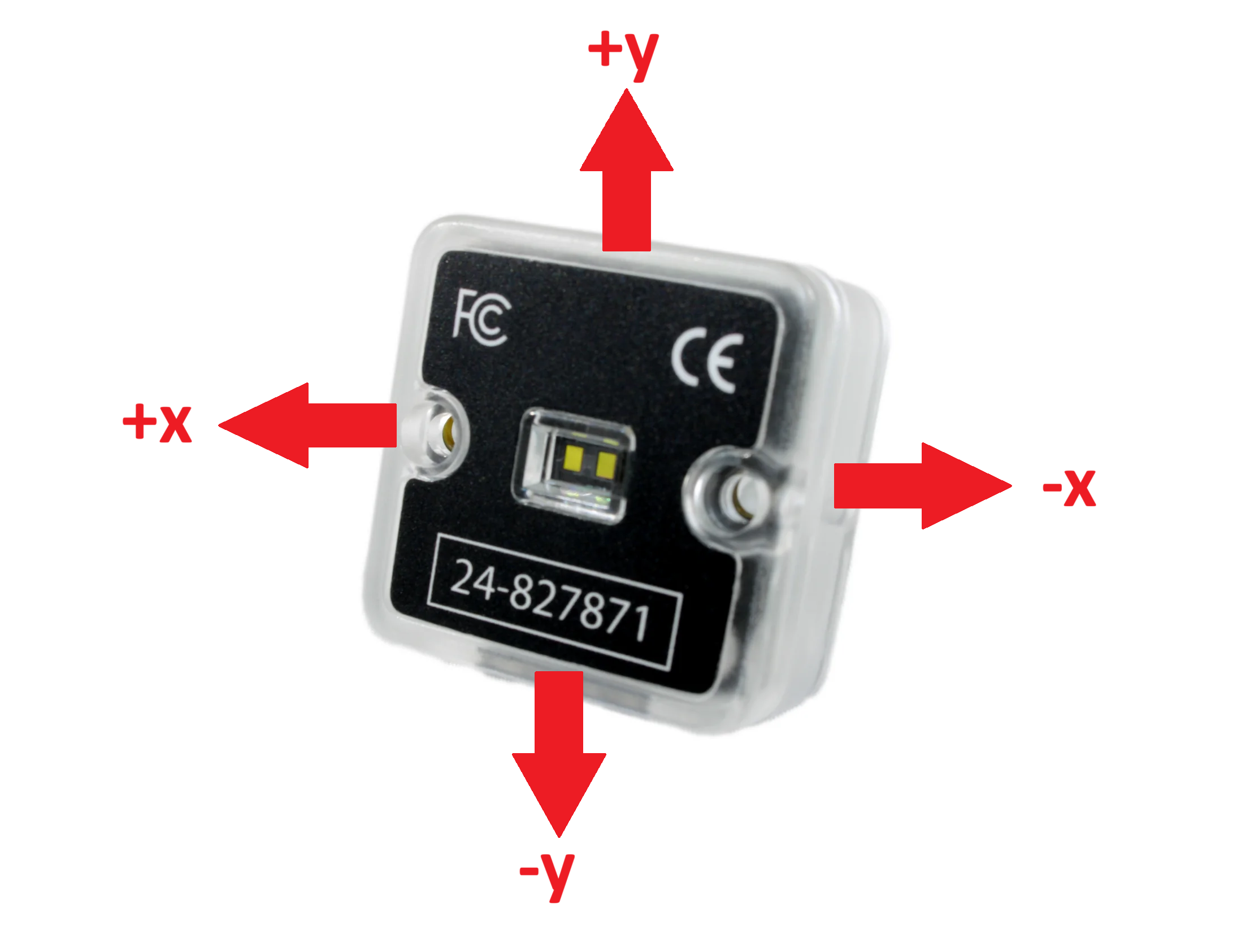
FOV CenterX / CenterY
These values (in degrees of rotation) are used to tell the CANrange where the center is and where it should be looking for objects.
-
-11° to 11°
FOV RangeX / RangeY
These values (also in degrees of rotation) are used to tell the CANrange how far away it should look from the center for objects
- 7° to 27°
|
Use this handy dandy image to check which directions are x, y, positive, and negative:
(The actual sensor part facing towards you) |
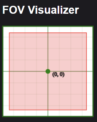
There is also an FOV Visualizer in Self Test that helps you see more clearly where the CANrange is looking: |
Min Signal Strength For Valid
This is set to 2500 as a default, and this a pretty good starting value. Check your plot for SignalStrength to see if you should adjust this value to be higher or lower.
Proximity Threshold
This is the most important value to tune! If the distance is less than this value, then the object is detected. Make sure you are plotting Distance on the graph, and then:
- Place an object in front of the CANrange and see the distance decrease on the plot → this is the minimum distance
- Remove the object from the CANrange and see the distance increase on the plot → this is the maximum distance
- Average the values of minimum and maximum distances together, and this is your new Proximity Threshold (in meters)
Proximity Hysteresis
This value (in meters) tells the CANrange the extra distance less from the Proximity Threshold before it recognizes the object as detected and the extra distance more before the object is no longer detected.
For example if the Proximity Threshold was 1.0m and the Proximity Hysteresis was 0.1m then
- When the distance is ≤ 0.9m, the object is detected
- When the distance is ≥ 1.1m, the object isn't detected anymore
Proximity Hysteresis is especially useful when the CANrange is detecting in a noisy environment, and it allows the distance to change quickly without it thinking it's no longer detected.
The Hysteresis should generally be a little bit less than the difference between your Threshold and your maximum/minimum
Your CANrange is now tuned! It's always a good idea to fiddle around with the values a little bit to get your desired output, but this is a great starting place!
Velocity Tuning with VelocityTorqueCurrentFOC
How to tune for Velocity
We like to use MotionMagic because it makes speed changes smoother! We use MotionMagic for basically all of our motion profiles.
When using a velocity profile, you are trying to get the motor to spin at a specific velocity instead of a rotating specific amount of rotations.
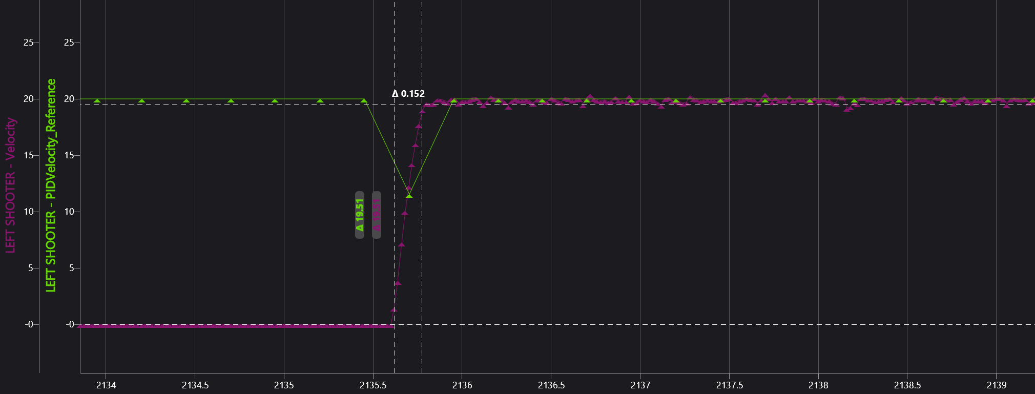
The Plot
|
In Phoenix Tuner, plot Velocity (rotations/sec) and Acceleration (rotations/sec2). |
|
Then also plot Reference (rotations/sec) and ReferenceSlope (rotations/sec2).
Make sure the Reference and ReferenceSlope are from PIDVelocity (not PIDPosition)
Gain Configurations
Motion Magic
-
Start with the MotionMagic configs
-
We don't use the cruise velocity gain in a velocity profile because we are trying to get to a target velocity, not this velocity we are setting
-
Make cruise acceleration 4, and double from there after more tuning
-
FeedForward and FeedBack
Try to minimize the amount of feedback gains while tuning, but use them if necessary
-
kS
-
Set to 1 and start doubling (use binary searching to get the optimum value)
-
We are trying to get the smallest kS possible before the motor starts turning
-
-
kA
-
Change it based on the Reference and our current Velocity signals
-
The steeper the slope of the Reference, the more we have to increase kA in order to get the Velocity to match it
-
A steeper slope means a higher kA and vice versa
-
-
kV
-
After getting the Velocity to peak along with Reference, it's time to raise kV
-
Increase kV until the Velocity line stays straight and is closely matching the Reference
-
These should get you pretty close to the Reference line - change kP and kD a little bit to get to your desired accuracy!
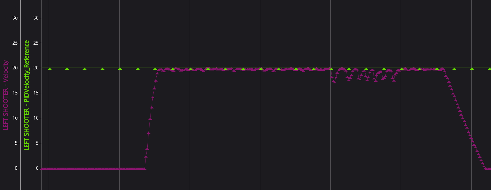
Specifics for Flywheel Tuning
While tuning flywheels, we are trying to get the motor to get to its target as fast as possible. When a game piece (such as a ball) goes through it, it should take as little time as possible to ramp back up to speed.
-
To do make the motor reach its target faster, keep on doubling the Cruise Acceleration until it reaches the speed quickly
-
For Rebuilt, we decided that less than a quarter second was optimal for reaching the target
-
Decrease kS and kA little by little until the initial ramp up speed matches the profile (doesn't have to be perfect)
-
-
To make the motor ramp back up quicker, you have to tune other gains a little more
-
If game pieces are going through in quick succession as the velocity slows down by a lot, then you need to increase kP and kD
-
Double kP a couple times until the motor doesn't dip as far down in velocity
-
If there is too much oscillation now, increase kD a little bit
-
-
Remember: kP makes the motor move faster if the error is bigger, and kD resists changes to the motor's velocity
-
-
For Rebuilt, we decided that less than a 10th of a second was good for the motor to ramp back up to speed
-
Shooting Our Shot
Shooting Our Shot - How to Create an Interpolating Tree Map
An Interpolating Tree Map (aka a Shooter Map) boiled down to its core is just linear regression. It was highly used during the Rebuilt Season for shooting into the hub and shuttling across the field.
For linear regression to work, it needs a bunch of data points. In the case of Rebuilt, the Shooter Map used the distance to the center of the hub as the input and it gave us the target rps for the shooter as the output.
Setting up the Map
To begin, you first need to manually find a bunch of good data points. We used the spots on the field where we would most often shoot from to determine our initial data points. Using these data points, we made a line graph on Google Sheets, and this helped us see where we were missing data. After this, we tested shooting with the shooter map automation and added in more data where the map failed.
The Code
The following are examples of code that was used during Rebuilt to setup our Shooter Map:
ShooterStateData.java in the util folder
package frc.robot.util;

import static edu.wpi.first.units.Units.Radians;

import edu.wpi.first.math.interpolation.Interpolator;
import edu.wpi.first.units.measure.Angle;

public class ShooterStateData {

    public static final Interpolator<ShooterStateData> interpolator = (startValue, endValue, t) -> {
        double initialHood = startValue.hoodPos.in(Radians);
        double finalHood = endValue.hoodPos.in(Radians);

        double initialRPS = startValue.rps;
        double finalRPS = endValue.rps;

        double initialToF = startValue.timeOfFlight;
        double finalToF = endValue.timeOfFlight;

        double interpolatedHood = initialHood + t * (finalHood - initialHood);

        return new ShooterStateData(
                Radians.of(interpolatedHood),
                initialRPS + t * (finalRPS - initialRPS),
                initialToF + t * (finalToF - initialToF));
    };
    public final Angle hoodPos;
    public final double rps;
    public final double timeOfFlight;

    public ShooterStateData(Angle hoodPos, double rps, double timeOfFlight) {
        this.hoodPos = hoodPos;
        this.rps = rps;
        this.timeOfFlight = timeOfFlight;
    }
}
Initializing the Shooter Map in ShooterConfigsBeta.java
public static final InterpolatingTreeMap<Double, ShooterStateData> SHOOTER_MAP =
            new InterpolatingTreeMap<>(InverseInterpolator.forDouble(), ShooterStateData.interpolator);
Logging Distance to Hub in Robot Container
public void updateLoggers() {
        Pose2d currentPose = drive.getState().Pose;
        Translation2d modifiedTarget = AllianceFlipUtil.apply(centerHubOpening.toTranslation2d());
        Translation2d currentPosition = currentPose.getTranslation();
        double distance = modifiedTarget.getDistance(currentPosition);

        Logger.recordOutput("AutoAimCommands/Shooter Map/hub distance", distance);
    }
Putting data into the Shooter Map (this is also in ShooterConfigsBeta.java, right underneath the initialization)
static {
        SHOOTER_MAP.put(1.74, new ShooterStateData(HoodPositions.STOW.getPosition(), 25, 0.0));
        SHOOTER_MAP.put(2.13, new ShooterStateData(HoodPositions.STOW.getPosition(), 27, 0.0));
        SHOOTER_MAP.put(2.43, new ShooterStateData(HoodPositions.STOW.getPosition(), 30, 0.0));
        SHOOTER_MAP.put(2.78, new ShooterStateData(HoodPositions.STOW.getPosition(), 31, 0.0));
        SHOOTER_MAP.put(3.15, new ShooterStateData(HoodPositions.STOW.getPosition(), 33, 0.0));
        SHOOTER_MAP.put(3.78, new ShooterStateData(HoodPositions.STOW.getPosition(), 38.7, 0.0));
        SHOOTER_MAP.put(4.36, new ShooterStateData(HoodPositions.STOW.getPosition(), 44, 0.0));
    }
Using the Shooter Map to actually calculate the target rps of the Shooter (in AutoAimCommands.java)
public static Command readyAim(CommandSwerveDrivetrain drive, Shooter shooter, Translation2d target) {

        return Commands.defer(
                () -> {
                    Pose2d currentPose = drive.getState().Pose;
                    Translation2d modifiedTarget = AllianceFlipUtil.apply(target);
                    Translation2d currentPosition = currentPose.getTranslation();
                    double distance = modifiedTarget.getDistance(currentPosition);

                    ShooterStateData state = ShooterConfigsBeta.SHOOTER_MAP.get(distance);

                    double targetRPS = state.rps;

                    Logger.recordOutput("AutoAimCommands/Shooter Map/target rps", targetRPS);

                    return shooter.shoot(targetRPS);
                },
                Set.of(shooter));
    }
The Shooter Map uses the distance to the hub the input, it does the linear regression, and then outputs the target rps.
Once you have set everything up, you'll be able to call the readyAim command using a controller binding and it'll work!
Position Tuning with MotionMagicTorqueCurrentFOC
This is a simple guide on how to tune MotionMagicTorqueCurrentFOC:
Firstly, and most importantly, find your maximum and minimum setpoints!!!!!
Put these as preset position rotations in Phoenix Tuner.
If you don't, your robot will break!
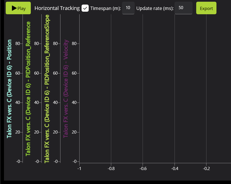
Signals:
Add the following signals to the plot:
- Position
- PID Position (Reference)
- Velocity
- PID Velocity (Reference Slope)
Create two groups to create uniform scales (feel free to change colors as necessary to increase visibility):
- Position & Position (Reference)
- Velocity & Velocity (Reference Slope)
Tuning:
Make sure your motors are working together:
To do this, move each motor in the mechanism separately with positive DutyCycle to find inversions.
- Zero all PID gains.
- Increase kG to find the smallest possible kG that stops the arm from moving.
- Increase kG and find the largest possible kG that stops the arm from moving.
- Set kG to the middle of the two values.
- Set kS to half the difference between the two values.
- Set a setpoint relatively small (typically 0.1 mechanism rotations).
- Increase kP until you notice significant overshoot.
If tuning a turret, start by finding kS by setting a small setpoint and finding the highest value that doesn't move the mechanism. Then continue from step 7 onwards.